  1
  2
  3
  4
  5
  6
  7
  8
  9
 10
 11
 12
 13
 14
 15
 16
 17
 18
 19
 20
 21
 22
 23
 24
 25
 26
 27
 28
 29
 30
 31
 32
 33
 34
 35
 36
 37
 38
 39
 40
 41
 42
 43
 44
 45
 46
 47
 48
 49
 50
 51
 52
 53
 54
 55
 56
 57
 58
 59
 60
 61
 62
 63
 64
 65
 66
 67
 68
 69
 70
 71
 72
 73
 74
 75
 76
 77
 78
 79
 80
 81
 82
 83
 84
 85
 86
 87
 88
 89
 90
 91
 92
 93
 94
 95
 96
 97
 98
 99
100
101
102
103
104
105
106
107
108
| # coding=utf-8
from math import exp
import matplotlib.pyplot as plt
import numpy as np
from sklearn.datasets.samples_generator import make_blobs
def sigmoid(num):
'''
:param num: 待计算的x
:return: sigmoid之后的数值
'''
if type(num) == int or type(num) == float:
return 1.0 / (1 + exp(-1 * num))
else:
raise ValueError, 'only int or float data can compute sigmoid'
class logistic():
def __init__(self, x, y):
if type(x) == type(y) == list:
self.x = np.array(x)
self.y = np.array(y)
elif type(x) == type(y) == np.ndarray:
self.x = x
self.y = y
else:
raise ValueError, 'input data error'
def sigmoid(self, x):
'''
:param x: 输入向量
:return: 对输入向量整体进行simgoid计算后的向量结果
'''
s = np.frompyfunc(lambda x: sigmoid(x), 1, 1)
return s(x)
def train_with_punish(self, alpha, errors, punish=0.0001):
'''
:param alpha: alpha为学习速率
:param errors: 误差小于多少时停止迭代的阈值
:param punish: 惩罚系数
:param times: 最大迭代次数
:return:
'''
self.punish = punish
dimension = self.x.shape[1]
self.theta = np.random.random(dimension)
compute_error = 100000000
times = 0
while compute_error > errors:
res = np.dot(self.x, self.theta)
delta = self.sigmoid(res) - self.y
self.theta = self.theta - alpha * np.dot(self.x.T, delta) - punish * self.theta # 带惩罚的梯度下降方法
compute_error = np.sum(delta)
times += 1
def predict(self, x):
'''
:param x: 给入新的未标注的向量
:return: 按照计算出的参数返回判定的类别
'''
x = np.array(x)
if self.sigmoid(np.dot(x, self.theta)) > 0.5:
return 1
else:
return 0
def test1():
'''
用来进行测试和画图,展现效果
:return:
'''
x, y = make_blobs(n_samples=200, centers=2, n_features=2, random_state=0, center_box=(10, 20))
x1 = []
y1 = []
x2 = []
y2 = []
for i in range(len(y)):
if y[i] == 0:
x1.append(x[i][0])
y1.append(x[i][1])
elif y[i] == 1:
x2.append(x[i][0])
y2.append(x[i][1])
# 以上均为处理数据,生成出两类数据
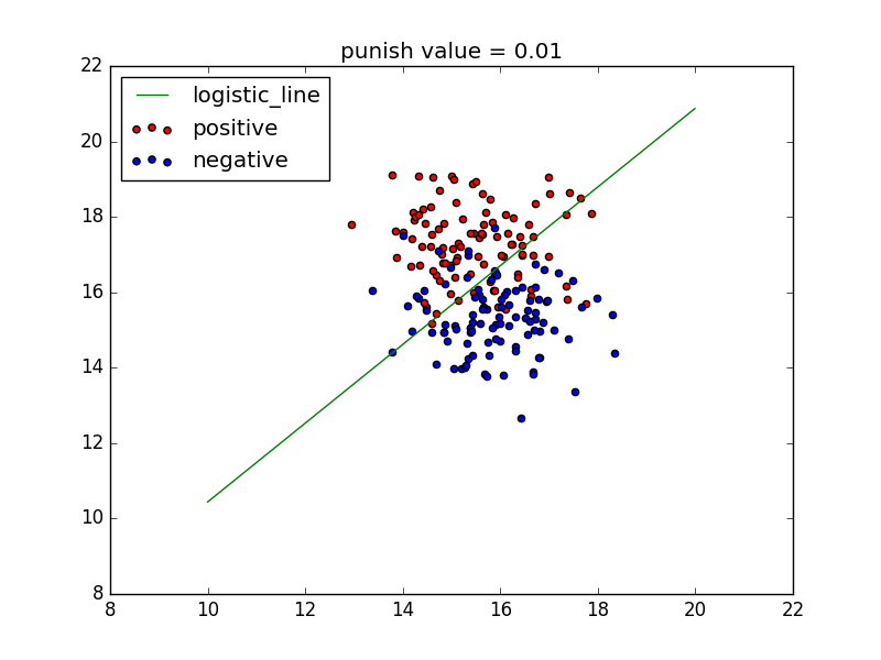
p = logistic(x, y)
p.train_with_punish(alpha=0.00001, errors=0.005, punish=0.01) # 步长是0.00001,最大允许误差是0.005,惩罚系数是0.01
x_test = np.arange(10, 20, 0.01)
y_test = (-1 * p.theta[0] / p.theta[1]) * x_test
plt.plot(x_test, y_test, c='g', label='logistic_line')
plt.scatter(x1, y1, c='r', label='positive')
plt.scatter(x2, y2, c='b', label='negative')
plt.legend(loc=2)
plt.title('punish value = ' + p.punish.__str__())
plt.show()
if __name__ == '__main__':
test1()
|