  1
  2
  3
  4
  5
  6
  7
  8
  9
 10
 11
 12
 13
 14
 15
 16
 17
 18
 19
 20
 21
 22
 23
 24
 25
 26
 27
 28
 29
 30
 31
 32
 33
 34
 35
 36
 37
 38
 39
 40
 41
 42
 43
 44
 45
 46
 47
 48
 49
 50
 51
 52
 53
 54
 55
 56
 57
 58
 59
 60
 61
 62
 63
 64
 65
 66
 67
 68
 69
 70
 71
 72
 73
 74
 75
 76
 77
 78
 79
 80
 81
 82
 83
 84
 85
 86
 87
 88
 89
 90
 91
 92
 93
 94
 95
 96
 97
 98
 99
100
101
102
103
104
105
106
107
108
109
110
111
112
113
114
115
116
117
118
119
120
121
122
123
124
125
126
127
128
129
130
131
132
133
134
135
136
137
138
139
140
141
142
143
144
145
146
147
148
149
150
151
152
153
154
155
156
157
158
159
160
161
162
163
164
165
166
167
168
169
170
| # coding=utf8
import random
import numpy as np
import tensorflow as tf
from sklearn import svm
right0 = 0.0 # 记录预测为1且实际为1的结果数
error0 = 0 # 记录预测为1但实际为0的结果数
right1 = 0.0 # 记录预测为0且实际为0的结果数
error1 = 0 # 记录预测为0但实际为1的结果数
for file_num in range(10):
# 在十个随机生成的不相干数据集上进行测试,将结果综合
print 'testing NO.%d dataset.......' % file_num
ff = open('digit_train_' + file_num.__str__() + '.data')
rr = ff.readlines()
x_test2 = []
y_test2 = []
for i in range(len(rr)):
x_test2.append(map(int, map(float, rr[i].split(' ')[:256])))
y_test2.append(map(int, rr[i].split(' ')[256:266]))
ff.close()
# 以上是读出训练数据
ff2 = open('digit_test_' + file_num.__str__() + '.data')
rr2 = ff2.readlines()
x_test3 = []
y_test3 = []
for i in range(len(rr2)):
x_test3.append(map(int, map(float, rr2[i].split(' ')[:256])))
y_test3.append(map(int, rr2[i].split(' ')[256:266]))
ff2.close()
# 以上是读出测试数据
sess = tf.InteractiveSession()
# 建立一个tensorflow的会话
# 初始化权值向量
def weight_variable(shape):
initial = tf.truncated_normal(shape, stddev=0.1)
return tf.Variable(initial)
# 初始化偏置向量
def bias_variable(shape):
initial = tf.constant(0.1, shape=shape)
return tf.Variable(initial)
# 二维卷积运算,步长为1,输出大小不变
def conv2d(x, W):
return tf.nn.conv2d(x, W, strides=[1, 1, 1, 1], padding='SAME')
# 池化运算,将卷积特征缩小为1/2
def max_pool_2x2(x):
return tf.nn.max_pool(x, ksize=[1, 2, 2, 1], strides=[1, 2, 2, 1], padding='SAME')
# 给x,y留出占位符,以便未来填充数据
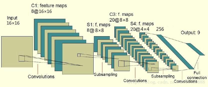
x = tf.placeholder("float", [None, 256])
y_ = tf.placeholder("float", [None, 10])
# 设置输入层的W和b
W = tf.Variable(tf.zeros([256, 10]))
b = tf.Variable(tf.zeros([10]))
# 计算输出,采用的函数是softmax(输入的时候是one hot编码)
y = tf.nn.softmax(tf.matmul(x, W) + b)
# 第一个卷积层,5x5的卷积核,输出向量是32维
w_conv1 = weight_variable([5, 5, 1, 32])
b_conv1 = bias_variable([32])
x_image = tf.reshape(x, [-1, 16, 16, 1])
# 图片大小是16*16,,-1代表其他维数自适应
h_conv1 = tf.nn.relu(conv2d(x_image, w_conv1) + b_conv1)
h_pool1 = max_pool_2x2(h_conv1)
# 采用的最大池化,因为都是1和0,平均池化没有什么意义
# 第二层卷积层,输入向量是32维,输出64维,还是5x5的卷积核
w_conv2 = weight_variable([5, 5, 32, 64])
b_conv2 = bias_variable([64])
h_conv2 = tf.nn.relu(conv2d(h_pool1, w_conv2) + b_conv2)
h_pool2 = max_pool_2x2(h_conv2)
# 全连接层的w和b
w_fc1 = weight_variable([4 * 4 * 64, 256])
b_fc1 = bias_variable([256])
# 此时输出的维数是256维
h_pool2_flat = tf.reshape(h_pool2, [-1, 4 * 4 * 64])
h_fc1 = tf.nn.relu(tf.matmul(h_pool2_flat, w_fc1) + b_fc1)
# h_fc1是提取出的256维特征,很关键。后面就是用这个输入到SVM中
#比方说,我训练完数据了,那么想要提取出来全连接层的h_fc1,
#那么使用的语句是sess.run(h_fc1, feed_dict={x: input_x}),返回的结果就是特征向量
# 设置dropout,否则很容易过拟合
keep_prob = tf.placeholder("float")
h_fc1_drop = tf.nn.dropout(h_fc1, keep_prob)
# 输出层,在本实验中只利用它的输出反向训练CNN,至于其具体数值我不关心
w_fc2 = weight_variable([256, 10])
b_fc2 = bias_variable([10])
y_conv = tf.nn.softmax(tf.matmul(h_fc1_drop, w_fc2) + b_fc2)
cross_entropy = -tf.reduce_sum(y_ * tf.log(y_conv))
# 设置误差代价以交叉熵的形式
train_step = tf.train.AdamOptimizer(1e-4).minimize(cross_entropy)
# 用adma的优化算法优化目标函数
correct_prediction = tf.equal(tf.argmax(y_conv, 1), tf.argmax(y_, 1))
accuracy = tf.reduce_mean(tf.cast(correct_prediction, "float"))
sess.run(tf.initialize_all_variables())
for i in range(3000):
# 跑3000轮迭代,每次随机从训练样本中抽出50个进行训练
batch = ([], [])
p = random.sample(range(795), 50)
for k in p:
batch[0].append(x_test2[k])
batch[1].append(y_test2[k])
if i % 100 == 0:
train_accuracy = accuracy.eval(feed_dict={x: batch[0], y_: batch[1], keep_prob: 1.0})
# print "step %d, train accuracy %g" % (i, train_accuracy)
train_step.run(feed_dict={x: batch[0], y_: batch[1], keep_prob: 0.6})
# 设置dropout的参数为0.6,测试得到,大点收敛的慢,小点出现过拟合
print "test accuracy %g" % accuracy.eval(feed_dict={x: x_test3, y_: y_test3, keep_prob: 1.0})
for h in range(len(y_test2)):
if np.argmax(y_test2[h]) == 7:
y_test2[h] = 1
else:
y_test2[h] = 0
for h in range(len(y_test3)):
if np.argmax(y_test3[h]) == 7:
y_test3[h] = 1
else:
y_test3[h] = 0
# 以上两步都是为了将源数据的one hot编码改为1和0,我的学号尾数为7
x_temp = []
for g in x_test2:
x_temp.append(sess.run(h_fc1, feed_dict={x: np.array(g).reshape((1, 256))})[0])
# 将原来的x带入训练好的CNN中计算出来全连接层的特征向量,将结果作为SVM中的特征向量
x_temp2 = []
for g in x_test3:
x_temp2.append(sess.run(h_fc1, feed_dict={x: np.array(g).reshape((1, 256))})[0])
clf = svm.SVC(C=0.9, kernel='rbf')
clf.fit(x_temp, y_test2)
# SVM选择了rbf核,C选择了0.9
for j in range(len(x_temp2)):
# 验证时出现四种情况分别对应四个变量存储
if clf.predict(x_temp2[j])[0] == y_test3[j] == 1:
right0 += 1
elif clf.predict(x_temp2[j])[0] == y_test3[j] == 0:
right1 += 1
elif clf.predict(x_temp2[j])[0] == 1 and y_test3[j] == 0:
error0 += 1
else:
error1 += 1
accuracy = right0 / (right0 + error0) # 准确率
recall = right0 / (right0 + error1) # 召回率
print 'svm right ratio ', (right0 + right1) / (right0 + right1 + error0 + error1) #分类的正确率
print 'accuracy ', accuracy
print 'recall ', recall
print 'F1 score ', 2 * accuracy * recall / (accuracy + recall) # F1值
|

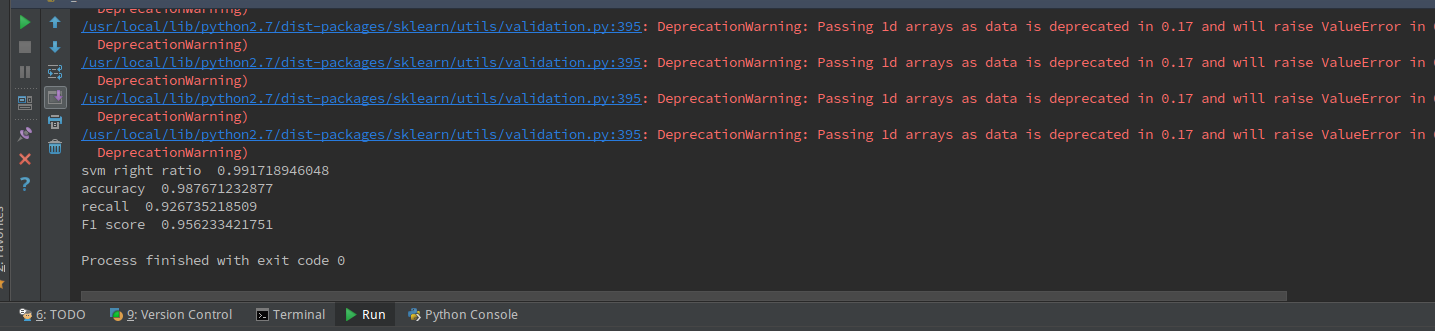 分类的正确率达到了99.1%,准确率98.77%,召回率为92.67%,F1值为0.9562
由于我们是十次验证取平均值,所以模型的泛化能力和准确度都还是比较令人满意的。
全部源代码和使用到的数据(按照前文规则生成的训练集和测试集)下载链接:/static/CNN-SVM.rar
分类的正确率达到了99.1%,准确率98.77%,召回率为92.67%,F1值为0.9562
由于我们是十次验证取平均值,所以模型的泛化能力和准确度都还是比较令人满意的。
全部源代码和使用到的数据(按照前文规则生成的训练集和测试集)下载链接:/static/CNN-SVM.rar